# Setting a CRAN mirror to avoid errors
options(repos = c(CRAN = "https://cloud.r-project.org/"))

# Install the required packages
# List of packages to check and install if missing
packages <- c(
  "priceR", "rvest", "dplyr", "googlesheets4",
  "rnaturalearth", "rnaturalearthdata", "sf",
  "xml2", "tidyverse"
)

# Loop through each package
for (pkg in packages) {
  if (!require(pkg, character.only = TRUE)) {
    install.packages(pkg)
    library(pkg, character.only = TRUE) # Load the package after installation
  }
}

library(dplyr)
library(tidyr)
library(ggplot2)
library(stringr)
library(rvest)
library(priceR)
library(rnaturalearth)
library(rnaturalearthdata)
library(sf)
library(rvest)
library(xml2)
library(tidyverse)
library(googlesheets4)
library(httr)
library(quantmod)
library(knitr)Olympics by Culture and Spending - The Olympic Advantage
Why do we care about the Olympics
For the purposes of this document I am going to encourage you to read the overall report that the team and I created on why we cared about the Olympics and what we sought out to figure out about the influences over the Olympics.
The main four components of the research were focused around:
- The country’s economy
- Investment and culture of sportiness (the individual report provided below with the research).
- Geographic characteristics
- Impact of being the host country
Country’s investment into sports culture
To provide the introduction to this, it’s important to know what I was most curious about when preparing and some of the topical questions that I sought to answer. So the areas I was focusing on:
- Sportiness of the population/culture, measured through:
- Elite Sports ranking
- Hobbies involving sports
- Watching Sport
- Health & Fitness
- Playing sport
- Sports Participation rate
- Financial Metrics of sportiness
- Fitness Applications
- Fitness Spend
- Gym memberships (per 100K)
- Overall country spending on sports related equipment
This prelude to the topic was what influences from culture and spending most impact the ability to win an Olympic medal for a country. Leading to what is the correlation and causation of the factors and number of Olympic medals won and what is the likeliness of it being chance.
To start the analysis, if you are curious to know what libraries were used in this investigation expand the code below to see the list, that were either utilized or tested whilst developing the code.
Relevant libraries
Geospatial Analysis
So the first source I went to for my data source, was Myprotein, and I know what you are thinking an odd location for a research database, however the Research by Adele Halsall provided a fascinating insight into overall sportiness especially in trying to measure sports culture which is never easy. She was kind enough to store her data on a google sheet, and as such that company with the googlesheets4 library meant I could extract into my table.
Pulling in MyProtein Sporties Country data
sheet_id <- "1JMS4D9Nx-qxokAkStZ-hJ9vCobphCVqWjZHSGsodlbE"
#this is the sheet utilized in googlesheets after the /spreadsheets/d/sheetid

gs4_deauth()
# As it is publically accessible do not need a google account

# Read the data with read_sheet pertaining to the googlesheets4 library
data <- read_sheet(sheet_id)

head(n = 10,data)
# A tibble: 10 × 12
Country `Olympic Medals` Winter Olympic Medal…¹ `Elite Sport Ranking`
<chr> <dbl> <dbl> <dbl>
1 Germany 1346 408 1
2 United States … 2522 305 7
3 Sweden 494 158 4
4 Norway 152 368 3
5 Finland 303 167 27
6 Canada 302 199 2
7 Switzerland 192 153 5
8 Austria 87 232 10
9 Netherlands 285 130 25
10 Australia 507 15 13
# ℹ abbreviated name: ¹`Winter Olympic Medals`
# ℹ 8 more variables: `Sports Participation Rate` <dbl>,
# `Gym Memberships per 100k` <dbl>, `Hobbies - Health & Fitness` <dbl>,
# `Hobbies - Playing Sport` <dbl>, `Hobbies - Watching Sport` <dbl>,
# `Fitness Apps` <dbl>, `Fitness Spend` <dbl>,
# `Total Score (out of 100)` <dbl>Now whilst the above was useful for getting the data for analysis we needed to also enhance the information with Geospatial information for the purposes of mapping the information.
Pulling in the world map
world <- ne_countries(scale = "medium", returnclass = "sf") |>
#This ne_countries is from the rnaturalearth library in R and contains country based information
  select(name) |>
  mutate(name = case_when(
    name == "Czechia" ~ "Czech Republic",
    name == "U.S. Virgin Is." ~ "Virgin Islands",
    name == "Côte d'Ivoire" ~ "Ivory Coast",
    name == "Dominican Rep." ~ "Dominican Republic",
    TRUE ~ name # Keep other values unchanged
    ))
#Tidied up the naming conventions of countries to align with the information provided in the MyProtein Sports review

ggplot(world) +
  geom_sf(aes(geometry = geometry)) +
  labs(title = "Geometries Plot", x = "Longitude", y = "Latitude")
#this is the same visualization as below and uses a native R libraryI have provided a visualization of the bare bones map provided in this analysis, the logic is hidden above in the code but want to share the insights generated.
Then after tidying everything up we combine the two pieces of data to present the information in a plotted format, instead of as a table, as a visual learner and observer it will help to make points clearer.
Data integration and mapping
merged_World_data <- inner_join(world,data, by = c("name" = "Country")) |>
      mutate(`Elite Sport Ranking` = 84-`Elite Sport Ranking`)
# the purpose of the mutate in this case is given that the lower the number the better the performance i.e. Country ranked 1st performs better we took the inverse of worst performing country for the Elite Sports ranking as this aligns with other metrics where higher is better.

ggplot(data = merged_World_data) +
  geom_sf(aes(fill = `Olympic Medals`)) + # Use the 'medals' column for fill color
  scale_fill_gradient(low = "lightblue", high = "darkblue", name = "Medals") + # Color gradient for medals
  theme_minimal() +
  labs(
    title = "Olympic Medals by Country",
    subtitle = "Visualizing the Number of Medals Won",
    caption = "MyProtein"
  )
#This is a duplication of the visualization naturally occuring however wanted to keep both so the code could be seen all together.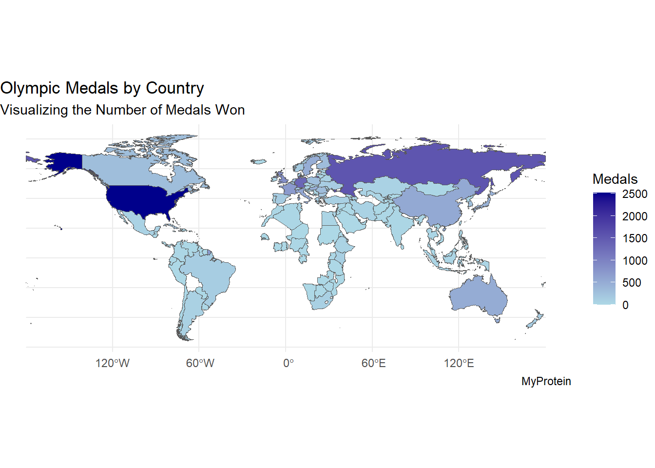
Next Compare each of the factors to analyse culture by mapping to each other of the 9 factors being (Olympic Medals, Winter Olympic Medals, Elite Sport Ranking, Sports Participation Rate, Gym Memberships per 100k, Hobbies - Health & Fitness, Hobbies - Watching Sport, Fitness Apps, Fitness Spend). The code below shows how it was cleaned and tidied to analyse a country comparison.
Tidying up Factors and presenting
long_data <- merged_World_data |>
  pivot_longer(
    cols = c(
      `Olympic Medals`, `Winter Olympic Medals`, `Elite Sport Ranking`,
      `Sports Participation Rate`, `Gym Memberships per 100k`,
      `Hobbies - Health & Fitness`, `Hobbies - Watching Sport`,
      `Fitness Apps`, `Fitness Spend`
    ),
    names_to = "Metric",
    values_to = "Value"
  ) |>
  group_by(Metric) %>%
  mutate(Normalized_Value = (Value - min(Value, na.rm = TRUE)) /
           (max(Value, na.rm = TRUE) - min(Value, na.rm = TRUE))) %>%
  ungroup()

# Plot using normalized values
ggplot(data = long_data) +
  geom_sf(aes(fill = Normalized_Value), color = "black") + # Fill with normalized value
  scale_fill_gradient(low = "lightblue", high = "darkblue", name = "Relative Value") +
  facet_wrap(~ Metric, ncol = 3) + # Use shared scales for geometry
  theme_minimal() +
  labs(
    title = "Comparison of Fitness and Sports Metrics by Country",
    subtitle = "Normalized Values by Metric"
  ) +
  theme(legend.position = "bottom")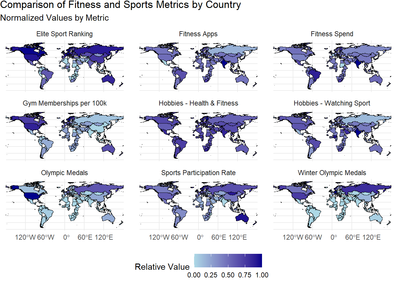
As you can see above the data shows a lot of correlations that can be visually observed before being analysed so some primary comments would be between the Gym Members per 100K and the Sports Participation rate.
As an aside and an Australian I will note that in all of these images we perform quite successfully except for the performance in Winter Olympic Medals, which is understandable especially living so close to the beach and water it is easier for summer sports.
Some notes for the top performer of the Number of Olympic medals of the U.S, it appears that the Elite Sports Ranking, Gym memberships per 100k and other factors quite evidently overlap, but I am interesting in hearing everyone thoughts on what other factors you would have included to account for the performance in the olympics.
The next section is more rigorous analytics around these factors and how they overlap by starting to quantify the regression with a causation and correlation focus of the supporting factors around the numbers of Olympic medals won. This is where the visualization of this data moves from graph to Table and the data enthusiasts start to really pay attention.
Regression
As mentioned below the first part is to ensure that the data quality is high and a successful regression analysis can be performed. This is largely analyzing the table above with some additional data cleansing and pivoting to allow it to flow into the data analytics format provided by the R libraries.
Regression code
Merged_unmapped_World_Data <- merged_World_data
#Creating a separate data table to remove the geometry or location for each country to reduce the data size

Merged_unmapped_World_Data$geometry <- NULL
#Setting the geometry to 0
y <- Merged_unmapped_World_Data$`Olympic Medals`
# Dependent variable

# Independent variables
X <- Merged_unmapped_World_Data |>
  select(
    `Elite Sport Ranking`,
    `Sports Participation Rate`,
    `Gym Memberships per 100k`,
    `Hobbies - Health & Fitness`,
    `Hobbies - Playing Sport`,
    `Hobbies - Watching Sport`,
    `Fitness Apps`,
    `Fitness Spend`
  )

# COmbining all the data
X <- cbind(X)
For the statistical analysis the Principal Component Analysis (PCA) was utilized across the data.
PCA Analysis
# This is possible because ot the stats library and so easily sharable
pca <- prcomp(X, scale. = TRUE)

# Use the first few principal components for regression
pca_data <- as.data.frame(pca$x[,1:8]) # Use the first 8 components
merged_data_pca <- cbind(y, pca_data)

# Fit the regression model
model_pca <- lm(y ~ ., data = merged_data_pca)

# Summarize the model code is suppressed below but used in a hidden run to show the table
summary(model_pca)
Call:
lm(formula = y ~ ., data = merged_data_pca)

Residuals:
    Min      1Q  Median      3Q     Max
-579.26 -103.39   -0.92   46.84 1677.87

Coefficients:
            Estimate Std. Error t value Pr(>|t|)
(Intercept)   115.06      20.66   5.568 1.50e-07 ***
PC1            74.32      13.12   5.663 9.68e-08 ***
PC2           -78.80      15.16  -5.200 7.91e-07 ***
PC3           -12.33      20.94  -0.589 0.557082
PC4           -79.48      24.12  -3.295 0.001281 **
PC5           -37.92      24.51  -1.547 0.124435
PC6           102.52      29.28   3.501 0.000643 ***
PC7            85.95      33.60   2.558 0.011717 *
PC8            57.80      37.26   1.552 0.123300
---
Signif. codes:  0 '***' 0.001 '**' 0.01 '*' 0.05 '.' 0.1 ' ' 1

Residual standard error: 239.2 on 125 degrees of freedom
Multiple R-squared:  0.429, Adjusted R-squared:  0.3925
F-statistic: 11.74 on 8 and 125 DF, p-value: 2.319e-12kable(pca$rotation[, 1:8])| PC1 | PC2 | PC3 | PC4 | PC5 | PC6 | PC7 | PC8 | |
|---|---|---|---|---|---|---|---|---|
| Elite Sport Ranking | 0.2552993 | -0.4660090 | 0.1369448 | -0.0525239 | -0.5938219 | 0.5032198 | 0.1898671 | -0.2328972 |
| Sports Participation Rate | 0.4068975 | -0.4114166 | 0.0458514 | 0.1075156 | 0.0144703 | -0.2951564 | -0.7509729 | -0.0148991 |
| Gym Memberships per 100k | 0.2073760 | -0.5255337 | 0.1684044 | -0.3650119 | 0.3755100 | -0.2805787 | 0.4702557 | 0.2798986 |
| Hobbies - Health & Fitness | -0.3451803 | -0.2808000 | 0.4469759 | 0.4093140 | 0.4742064 | 0.2136865 | -0.0141170 | -0.4048995 |
| Hobbies - Playing Sport | -0.3299214 | 0.0866252 | 0.6851963 | -0.1185995 | -0.4554738 | -0.4245194 | -0.0453082 | 0.1017949 |
| Hobbies - Watching Sport | -0.4549719 | -0.1670587 | -0.0248454 | -0.5726510 | 0.1090661 | 0.4300852 | -0.4107180 | 0.2664349 |
| Fitness Apps | -0.4034741 | -0.2929198 | -0.4573991 | -0.2066119 | -0.1442053 | -0.4106815 | 0.0539816 | -0.5541982 |
| Fitness Spend | -0.3584182 | -0.3705714 | -0.2677146 | 0.5479293 | -0.2028292 | -0.0376422 | 0.0706709 | 0.5610389 |
model_refined <- lm(y ~ PC1 + PC2 + PC4 + PC6 + PC7, data = merged_data_pca)
summary(model_refined)
Call:
lm(formula = y ~ PC1 + PC2 + PC4 + PC6 + PC7, data = merged_data_pca)

Residuals:
    Min      1Q  Median      3Q     Max
-650.21 -101.61   -4.96   48.21 1691.77

Coefficients:
            Estimate Std. Error t value Pr(>|t|)
(Intercept)   115.06      20.84   5.522 1.79e-07 ***
PC1            74.32      13.23   5.616 1.16e-07 ***
PC2           -78.80      15.28  -5.156 9.31e-07 ***
PC4           -79.48      24.32  -3.268 0.001392 **
PC6           102.52      29.53   3.472 0.000705 ***
PC7            85.95      33.88   2.537 0.012383 *
---
Signif. codes:  0 '***' 0.001 '**' 0.01 '*' 0.05 '.' 0.1 ' ' 1

Residual standard error: 241.2 on 128 degrees of freedom
Multiple R-squared:  0.4055,    Adjusted R-squared:  0.3823
F-statistic: 17.46 on 5 and 128 DF, p-value: 3.725e-13plot(model_refined$fitted.values, residuals(model_refined), xlab = "Fitted Values", ylab = "Residuals")
abline(h = 0, col = "red")qqnorm(residuals(model_refined))
qqline(residuals(model_refined), col = "red")In defining the Principal components we can see the regression provided below, and so to talk to some of the key numbers that are present, focusing below on the variables where the “loading” listed indicated the correlation or contribution of each variable to each principal component. With the following being true
A high positive loading (close to +1) means the variable is strongly positively correlated with the component.
A high negative loading (close to -1) means the variable is strongly negatively correlated with the component.
A loading close to 0 indicates a weak relationship.
| PC1 | PC2 | PC3 | PC4 | PC5 | PC6 | PC7 | PC8 | |
|---|---|---|---|---|---|---|---|---|
| Elite Sport Ranking | 0.26 | -0.47 | 0.14 | -0.05 | -0.59 | 0.50 | 0.19 | -0.23 |
| Sports Participation Rate | 0.41 | -0.41 | 0.05 | 0.11 | 0.01 | -0.30 | -0.75 | -0.01 |
| Gym Memberships per 100k | 0.21 | -0.53 | 0.17 | -0.37 | 0.38 | -0.28 | 0.47 | 0.28 |
| Hobbies - Health & Fitness | -0.35 | -0.28 | 0.45 | 0.41 | 0.47 | 0.21 | -0.01 | -0.40 |
| Hobbies - Playing Sport | -0.33 | 0.09 | 0.69 | -0.12 | -0.46 | -0.42 | -0.05 | 0.10 |
| Hobbies - Watching Sport | -0.45 | -0.17 | -0.02 | -0.57 | 0.11 | 0.43 | -0.41 | 0.27 |
| Fitness Apps | -0.40 | -0.29 | -0.46 | -0.21 | -0.14 | -0.41 | 0.05 | -0.55 |
| Fitness Spend | -0.36 | -0.37 | -0.27 | 0.55 | -0.20 | -0.04 | 0.07 | 0.56 |
This is where the analysis of probability of explanation comes into play, particularly noticed by the Pr(>|t|) value and the R-squared adding some context to the explanation. With the importance of the Principal components defined by the signif. codes to show how explainable it was.
Again this is primarily focused on the coding for the analysis however part of analyzing any good data source is the statistics behind it and as such I won’t talk in too much depth, however provided is the statistics behind the claims made (enjoy).
Call:
lm(formula = y ~ ., data = merged_data_pca)

Residuals:
    Min      1Q  Median      3Q     Max
-579.26 -103.39   -0.92   46.84 1677.87

Coefficients:
            Estimate Std. Error t value Pr(>|t|)
(Intercept)   115.06      20.66   5.568 1.50e-07 ***
PC1            74.32      13.12   5.663 9.68e-08 ***
PC2           -78.80      15.16  -5.200 7.91e-07 ***
PC3           -12.33      20.94  -0.589 0.557082
PC4           -79.48      24.12  -3.295 0.001281 **
PC5           -37.92      24.51  -1.547 0.124435
PC6           102.52      29.28   3.501 0.000643 ***
PC7            85.95      33.60   2.558 0.011717 *
PC8            57.80      37.26   1.552 0.123300
---
Signif. codes:  0 '***' 0.001 '**' 0.01 '*' 0.05 '.' 0.1 ' ' 1

Residual standard error: 239.2 on 125 degrees of freedom
Multiple R-squared:  0.429, Adjusted R-squared:  0.3925
F-statistic: 11.74 on 8 and 125 DF,  p-value: 2.319e-12
Next stages would be looking at the refined table by removing non critical factors these would be the values where Pr(>|t|) is higher than its counterparts or closer to 1 which indicates that the relationship is higher likelihood of being based on chance than actual relationship. The removed data would be PC3,5 and 8 and result in the below Regression analysis resulting in an Adjusted R-Squared value of 0.38 which is not the greatest explanation however given that this is a macro level view (i.e. country) and focusing on sports culture a social science it is a reasonable rate.
Call:
lm(formula = y ~ PC1 + PC2 + PC4 + PC6 + PC7, data = merged_data_pca)

Residuals:
    Min      1Q  Median      3Q     Max
-650.21 -101.61   -4.96   48.21 1691.77

Coefficients:
            Estimate Std. Error t value Pr(>|t|)
(Intercept)   115.06      20.84   5.522 1.79e-07 ***
PC1            74.32      13.23   5.616 1.16e-07 ***
PC2           -78.80      15.28  -5.156 9.31e-07 ***
PC4           -79.48      24.32  -3.268 0.001392 **
PC6           102.52      29.53   3.472 0.000705 ***
PC7            85.95      33.88   2.537 0.012383 *
---
Signif. codes:  0 '***' 0.001 '**' 0.01 '*' 0.05 '.' 0.1 ' ' 1

Residual standard error: 241.2 on 128 degrees of freedom
Multiple R-squared:  0.4055,    Adjusted R-squared:  0.3823
F-statistic: 17.46 on 5 and 128 DF,  p-value: 3.725e-13
So some of the key takeaways across the data focusing on three of the variables:
Elite Sport Ranking - Countries with strong elite sport rankings tend to perform better
Sports Participation rate - Higher Sports participation rate correlate with better olympic results
Hobbies - Health & Fitness - Countries where most people focus on personal fitness as a hobby may see indirect benefits in Olympic results.
Population Sport Spending
The next component of investigation was spending in Sports at the Retail Value RSP in local currency for each country. For this data Euromonitor, does a great job of consolidating this information so that it is easier to do an analysis and uses a variety of sources such as the SEC & IRS for the U.S numbers as official sources and many more. The first part of this was to normalize the numbers as they were in local currencies and aggregated in different capacity (some in millions, others in billions).
Euromonitor Sports Spend file read
Sports_spend <- read.csv("Passport_Stats_10-12-2024_0544_GMT.csv", skip = 5, header = TRUE) |>
  mutate(Currency =  substr(Unit, 1, 3)) |>
  mutate(X2023 = str_replace_all(X2023, ",", "")) |>
  mutate(X2023 = as.numeric(X2023)) |>
  filter(!is.na(Category) & Category != "")
#Given that Euromonitor does not have an API, and the shared license makes it difficult to parse the information, I downloaded and uploaded the information and focused on 2023

head(n = 5, Sports_spend)
Geography Category Data.Type Unit
1 China Outdoor and Sports Retail Value RSP CNY million
2 Hong Kong, China Outdoor and Sports Retail Value RSP HKD million
3 India Outdoor and Sports Retail Value RSP INR million
4 Indonesia Outdoor and Sports Retail Value RSP IDR billion
5 Japan Outdoor and Sports Retail Value RSP JPY billion
Current.Constant X2023 Currency
1 Current Prices 2458.7 CNY
2 Current Prices 70.3 HKD
3 Current Prices 1203.7 INR
4 Current Prices 211.7 IDR
5 Current Prices 13.1 JPYExtract FX rates
unique_currencies <- Sports_spend |>
  distinct(Currency) |>   # Get unique currencies
  pull(Currency)

# Combine the unique currencies into a comma-separated string
currency_string <- paste(unique_currencies, collapse = ",")

#Setting up an api key for the extract of Exchange Rates
Exchange_rate_api <- readLines("exchange rates api.txt")

#Downloading the exchange rates from the provided API
Exchange_rate_url <- paste0("https://api.exchangeratesapi.io/v1/2023-12-31?access_key=",Exchange_rate_api,"&symbols=",currency_string,"&format=1")

#Download the information
Exchange_rate <- GET(Exchange_rate_url)

#Parse the information
Usable_Exchange <- content(Exchange_rate, "parsed")

rates_table <- as_tibble(Usable_Exchange$rates)

long_data <- rates_table |>
  pivot_longer(
    cols = everything(),    # Select all columns
    names_to = "Currency",  # New column for the headers
    values_to = "Value"     # New column for the values
  )
#Setting it up as USD related focus of investment

USD_Value <- long_data |>
  filter(Currency == "USD") |>
  pull(Value)

Rates <- long_data |>
  mutate(Value_USD = as.numeric(1/(Value/USD_Value)))
#Converting everything to USD

Sports_spend <- Sports_spend |>
  left_join(Rates,Sports_spend, by = ("Currency"))
#Joining in the amount spent for Sports with the local currency adjustment to USD.

Sports_spend <- Sports_spend |>
  mutate(X2023_USD = X2023*Value_USD,
         Last7 = str_sub(Unit, -7),  # Extract the last 7 characters i.e. million or billion
         Multiplier = ifelse(Last7 == "million", 1000000, 1000000000), # Set multiplier based on condition
         X2023_USD = X2023_USD*Multiplier)

kable(Sports_spend)| Geography | Category | Data.Type | Unit | Current.Constant | X2023 | Currency | Value | Value_USD | X2023_USD | Last7 | Multiplier |
|---|---|---|---|---|---|---|---|---|---|---|---|
| China | Outdoor and Sports | Retail Value RSP | CNY million | Current Prices | 2458.7 | CNY | 7.825079 | 0.1412709 | 347342777 | million | 1e+06 |
| Hong Kong, China | Outdoor and Sports | Retail Value RSP | HKD million | Current Prices | 70.3 | HKD | 8.632571 | 0.1280564 | 9002365 | million | 1e+06 |
| India | Outdoor and Sports | Retail Value RSP | INR million | Current Prices | 1203.7 | INR | 92.027926 | 0.0120122 | 14459061 | million | 1e+06 |
| Indonesia | Outdoor and Sports | Retail Value RSP | IDR billion | Current Prices | 211.7 | IDR | 17013.075723 | 0.0000650 | 13755598 | billion | 1e+09 |
| Japan | Outdoor and Sports | Retail Value RSP | JPY billion | Current Prices | 13.1 | JPY | 155.900774 | 0.0070908 | 92889042 | billion | 1e+09 |
| Malaysia | Outdoor and Sports | Retail Value RSP | MYR million | Current Prices | 77.7 | MYR | 5.079529 | 0.2176296 | 16909822 | million | 1e+06 |
| Philippines | Outdoor and Sports | Retail Value RSP | PHP million | Current Prices | 474.9 | PHP | 61.238406 | 0.0180517 | 8572742 | million | 1e+06 |
| Singapore | Outdoor and Sports | Retail Value RSP | SGD million | Current Prices | 12.2 | SGD | 1.458677 | 0.7578484 | 9245750 | million | 1e+06 |
| South Korea | Outdoor and Sports | Retail Value RSP | KRW billion | Current Prices | 15.1 | KRW | 1431.045823 | 0.0007725 | 11664466 | billion | 1e+09 |
| Taiwan | Outdoor and Sports | Retail Value RSP | TWD million | Current Prices | 330.1 | TWD | 33.919310 | 0.0325908 | 10758209 | million | 1e+06 |
| Thailand | Outdoor and Sports | Retail Value RSP | THB million | Current Prices | 347.6 | THB | 38.066335 | 0.0290403 | 10094392 | million | 1e+06 |
| Australia | Outdoor and Sports | Retail Value RSP | AUD million | Current Prices | 133.7 | AUD | 1.622777 | 0.6812125 | 91078113 | million | 1e+06 |
| Poland | Outdoor and Sports | Retail Value RSP | PLN million | Current Prices | 202.3 | PLN | 4.344490 | 0.2544501 | 51475259 | million | 1e+06 |
| Romania | Outdoor and Sports | Retail Value RSP | RON million | Current Prices | 51.8 | RON | 4.978393 | 0.2220508 | 11502230 | million | 1e+06 |
| Russia | Outdoor and Sports | Retail Value RSP | RUB million | Current Prices | 14083.7 | RUB | 98.661662 | 0.0112045 | 157801018 | million | 1e+06 |
| Ukraine | Outdoor and Sports | Retail Value RSP | UAH million | Current Prices | 211.2 | UAH | 42.111813 | 0.0262505 | 5544105 | million | 1e+06 |
| Argentina | Outdoor and Sports | Retail Value RSP | ARS million | Current Prices | 7867.7 | ARS | 896.324454 | 0.0012333 | 9703402 | million | 1e+06 |
| Brazil | Outdoor and Sports | Retail Value RSP | BRL million | Current Prices | 422.6 | BRL | 5.364221 | 0.2060795 | 87089198 | million | 1e+06 |
| Mexico | Outdoor and Sports | Retail Value RSP | MXN million | Current Prices | 1182.3 | MXN | 18.764278 | 0.0589128 | 69652594 | million | 1e+06 |
| South Africa | Outdoor and Sports | Retail Value RSP | ZAR million | Current Prices | 536.9 | ZAR | 20.224535 | 0.0546592 | 29346500 | million | 1e+06 |
| United Arab Emirates | Outdoor and Sports | Retail Value RSP | AED million | Current Prices | 75.5 | AED | 4.060068 | 0.2722752 | 20556781 | million | 1e+06 |
| Canada | Outdoor and Sports | Retail Value RSP | CAD million | Current Prices | 210.8 | CAD | 1.464723 | 0.7547202 | 159095013 | million | 1e+06 |
| USA | Outdoor and Sports | Retail Value RSP | USD million | Current Prices | 1985.5 | USD | 1.105456 | 1.0000000 | 1985500000 | million | 1e+06 |
| France | Outdoor and Sports | Retail Value RSP | EUR million | Current Prices | 356.6 | EUR | 1.000000 | 1.1054560 | 394205610 | million | 1e+06 |
| Germany | Outdoor and Sports | Retail Value RSP | EUR million | Current Prices | 176.6 | EUR | 1.000000 | 1.1054560 | 195223530 | million | 1e+06 |
| Italy | Outdoor and Sports | Retail Value RSP | EUR million | Current Prices | 90.8 | EUR | 1.000000 | 1.1054560 | 100375405 | million | 1e+06 |
| Netherlands | Outdoor and Sports | Retail Value RSP | EUR million | Current Prices | 57.5 | EUR | 1.000000 | 1.1054560 | 63563720 | million | 1e+06 |
| Spain | Outdoor and Sports | Retail Value RSP | EUR million | Current Prices | 84.9 | EUR | 1.000000 | 1.1054560 | 93853214 | million | 1e+06 |
| Sweden | Outdoor and Sports | Retail Value RSP | SEK million | Current Prices | 397.2 | SEK | 11.152225 | 0.0991243 | 39372154 | million | 1e+06 |
| Switzerland | Outdoor and Sports | Retail Value RSP | CHF million | Current Prices | 58.1 | CHF | 0.929683 | 1.1890677 | 69084832 | million | 1e+06 |
| Turkey | Outdoor and Sports | Retail Value RSP | TRY million | Current Prices | 386.3 | TRY | 32.463169 | 0.0340526 | 13154528 | million | 1e+06 |
| United Kingdom | Outdoor and Sports | Retail Value RSP | GBP million | Current Prices | 162.4 | GBP | 0.868386 | 1.2730007 | 206735316 | million | 1e+06 |
Aggregated USD amount spent on sports equipment in 2023 for 34 countries, to provide some context as to how much each country spends on sports. This will be cross referenced against the number of medals won.
| Geography | USD Amount |
|---|---|
| USA | 1985500000 |
| France | 394205610 |
| China | 347342777 |
| United Kingdom | 206735316 |
| Germany | 195223530 |
| Canada | 159095013 |
| Russia | 157801018 |
| Italy | 100375405 |
| Spain | 93853214 |
| Japan | 92889042 |
| Australia | 91078113 |
| Brazil | 87089198 |
| Mexico | 69652594 |
| Switzerland | 69084832 |
| Netherlands | 63563720 |
| Poland | 51475259 |
| Sweden | 39372154 |
| South Africa | 29346500 |
| United Arab Emirates | 20556781 |
| Malaysia | 16909822 |
| India | 14459061 |
| Indonesia | 13755598 |
| Turkey | 13154528 |
| South Korea | 11664466 |
| Romania | 11502230 |
| Taiwan | 10758209 |
| Thailand | 10094392 |
| Argentina | 9703402 |
| Singapore | 9245750 |
| Hong Kong, China | 9002365 |
| Philippines | 8572742 |
| Ukraine | 5544105 |
After all of this sports spend we tie it back to the original question which is how does sports spending relate to Olympic medals won, we join the legacy data of Olympic medals to the new sport spend data that was listed above.
It is interesting to compare the R-squared values in the Olympic medal regression analysis where this model of current spend (i.e. 2023 USD in millions) is a better estimator of winning an Olympic medal compared to the previous analysis focused on hobbies and International sports ranking. The confidence P-value is indicative of this, feel free to further dive into the data below.
Regression of Medals to Amount spent
Sports_spend_medals <- Sports_spend |>
  mutate(Geography = case_when(
    Geography == "USA" ~ "United States of America",
    Geography == "Hong Kong, China" ~ "Hong Kong",
    TRUE ~ Geography)) |>
  mutate(X2023_USD = X2023_USD/1000000) |>
  left_join(data |>
              select(`Olympic Medals`,Country), by = c("Geography" = "Country"))

model <- lm(`Olympic Medals` ~ X2023_USD, data = Sports_spend_medals)

# Display the summary of the regression model (code suppressed here and hidden overall)
summary(model)
Call:
lm(formula = `Olympic Medals` ~ X2023_USD, data = Sports_spend_medals)

Residuals:
    Min      1Q  Median      3Q     Max
-227.21 -189.68 -115.48   58.82 1153.54

Coefficients:
            Estimate Std. Error t value Pr(>|t|)
(Intercept) 203.2603    60.9761   3.333  0.00229 **
X2023_USD     1.2624     0.1642   7.689 1.41e-08 ***
---
Signif. codes:  0 '***' 0.001 '**' 0.01 '*' 0.05 '.' 0.1 ' ' 1

Residual standard error: 320.4 on 30 degrees of freedom
Multiple R-squared:  0.6634,    Adjusted R-squared:  0.6521
F-statistic: 59.11 on 1 and 30 DF,  p-value: 1.412e-08
To further cement all of this, a graph has been provided below with 95% confidence intervals to highlight the data spent, obviously this is difficult due to the closer grouping of the data to the under $250 million USD spent on sport related items. Further analysis could definitely be performed here to complete a logarithmic analysis or some alternative type.
Plotting Spend vs Olympic medals
# Extract the formula
formula_text <- paste0("y = ", round(coef(model)[1], 2),
                       " + ", round(coef(model)[2], 2), "x")


ggplot(Sports_spend_medals, aes(x = X2023_USD, y = `Olympic Medals`)) +
  geom_point(color = "blue", size = 3) +
  geom_smooth(method = "lm", color = "red", se = TRUE) +
  annotate("text", x = 1000, y = 2000, label = formula_text, color = "black", size = 5, hjust = 0) +
  labs(
  title = "Sports Spending vs Olympic Medals",
  x = "Sports Spending in 2023 (Million USD)",
  y = "Olympic Medals"
  ) +
  theme_minimal()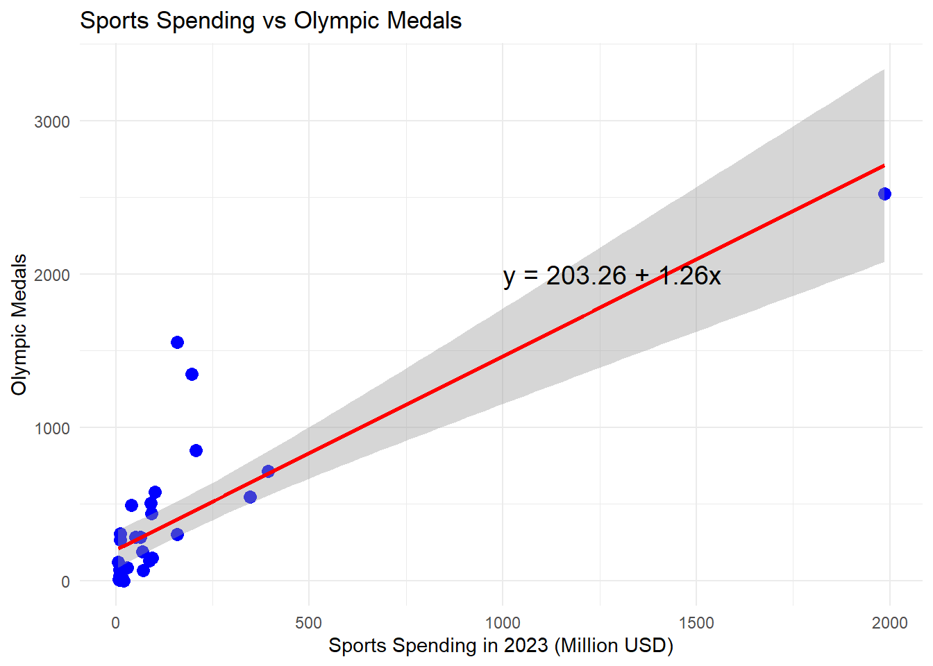
All of this shows the more that a country spends the more Olympic medals that are won with it only costing roughly a million USD for population per medal won.
Thank you for reading the analysis, I would highly recommend again reviewing my colleagues research into the other 4 components or the over-view non technical analysis. Otherwise feel free to connect via Linkedin to discuss this topic further, or generally to talk about coding, financial services or low-code no code tools as that is my specialty.
References:
Halsall, A. (2021, July 8). Which are the world’s sportiest countries? - MYPROTEINTM. MYPROTEIN. https://us.myprotein.com/thezone/motivation/which-are-the-worlds-sportiest-countries/
Euromonitor International. (2022). Outdoor and sports market size dataset. [Data file]. Retrieved from https://www.euromonitor.com
Exchange Rates API. (n.d.). Documentation. Retrieved from https://exchangeratesapi.io/documentation